SynDiag - Synthetic Diagnostics
SynDiag - Synthetic Diagnostics using MATLAB_edu module
SynDiag is a tool for simulating diagnostics given a reference plasma scenario and a geometry configuration. You can use it with the SimPla output or with a plasma configuration which is in SimPla format.
MATLAB Guide
In case you need to simulate diagnostics in a plasma scenario, please open Main_Diagnostics.m. The code “Main_Diagnostics.mat” allows for the design of the diagnostics setup. The current version includes the design of magnetic coils (pick-up, flux loops, and saddle loops), Thomson Scattering, and Interferometer-Polarimeter. The standard configuration is shown in Figure 1.
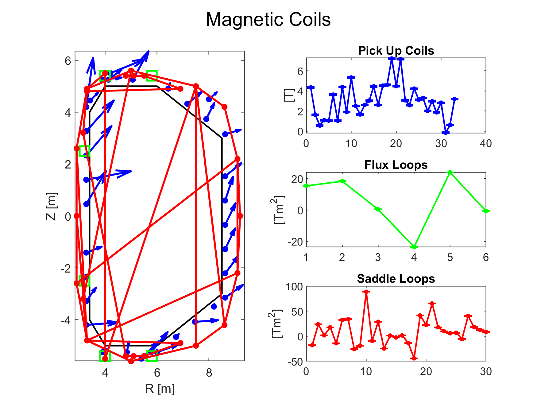
The configuration provided by TokaLab is denoted as “Configuration 1.” It is characterized by the quantities shown in Figure 1, where each measurement is Gaussian distributed with noise having a standard deviation of 10% of the standard deviation of measurements of the same kind (but ideal values are always accessible in the “ideal” substructure of each diagnostic structure). Each user can add their own configuration by varying the number of diagnostics, their location, and their measurement uncertainty. In this document, a brief comment on the code is first provided, and the TokaLab configuration for diagnostics is shown. Examples are then presented to demonstrate how to change the hyperparameters. It is first necessary to load an equilibrium (available through the execution of Main_Equilibrium.mat, for which users can find documentation in the dedicated section) and the file containing information on the geometry. For the provided configuration, magnetic diagnostics data are loaded through MATLAB files. These files contain information about the location of the coils and, for pick-up coils, information on their unit vector describing the coils’ orientation. Each diagnostic is then treated within a specific code section. Users can change the location or number of diagnostics by loading a file containing the desired information of this type and then adding another else if condition (with configuration == i, i > 1), copying the content of the first case and modifying the noise level, for example. For Thomson Scattering and Interferometer-Polarimeter, no file needs to be loaded before running the code. However, information related to the position of the diagnostics can be changed in the ThomsonScattering.m or InterferometerPolarimeter.m functions in the very first lines. All the following examples relate to the use of noisy measurements.
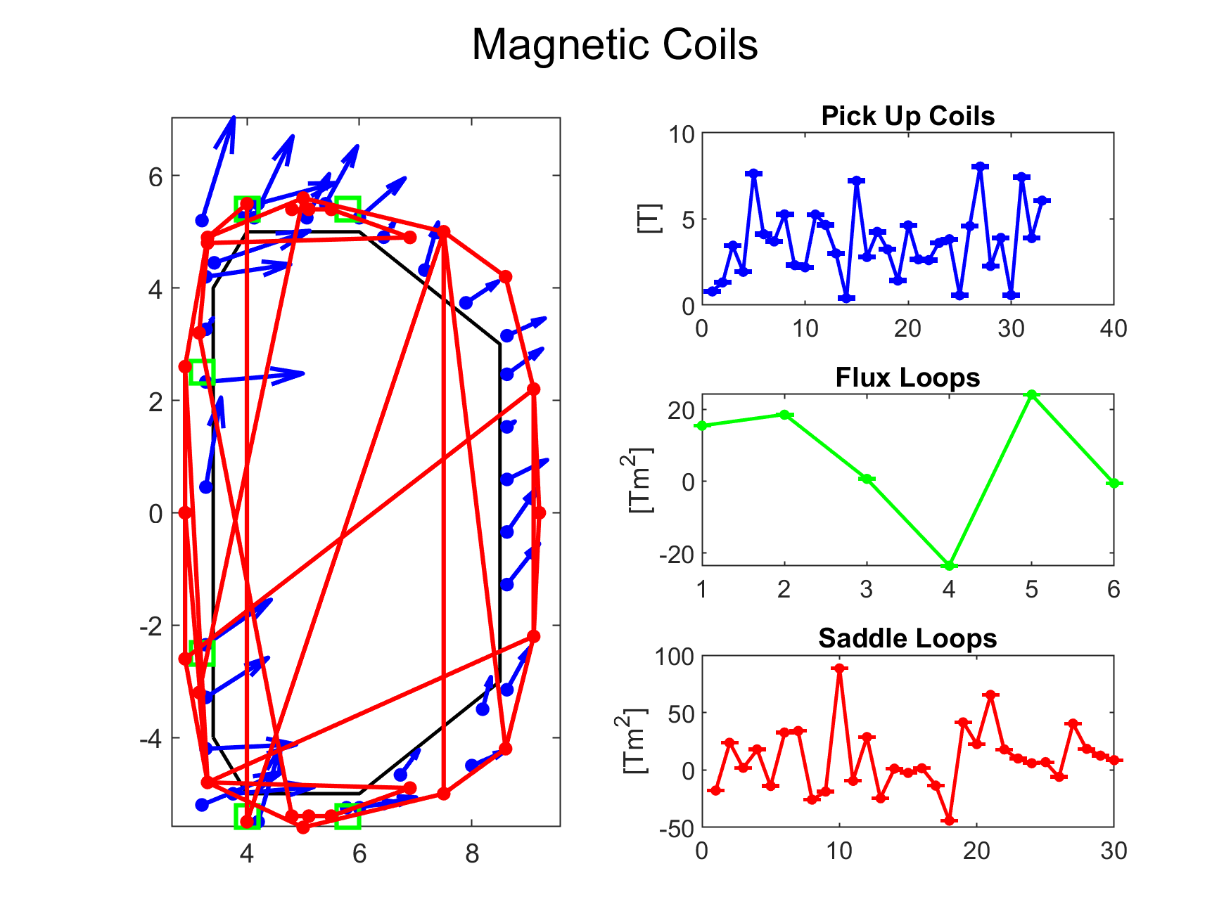
EXAMPLE 1: Modifying Pick Up Coils location an dorientation
Modifying Pick-Up coils location and orientation can be done by loading a file that simply contains information on R, z, and the poloidal angle in the same format provided through the standard configuration setting of the pick-up coils (a horizontal vector for R, a horizontal vector for Z, and a 3 x i matrix, with i = number of pick-up coils, indicating the components of the unit vector describing the coil orientation). In our case we used a MATLAB file, but a .txt or other format can be used by just modifying the loading function in line 6 of PickUpCoils.m (and the same for FluxLoops.m and SaddleLoops.m). An example of the new configuration obtained is shown in Figure 2.
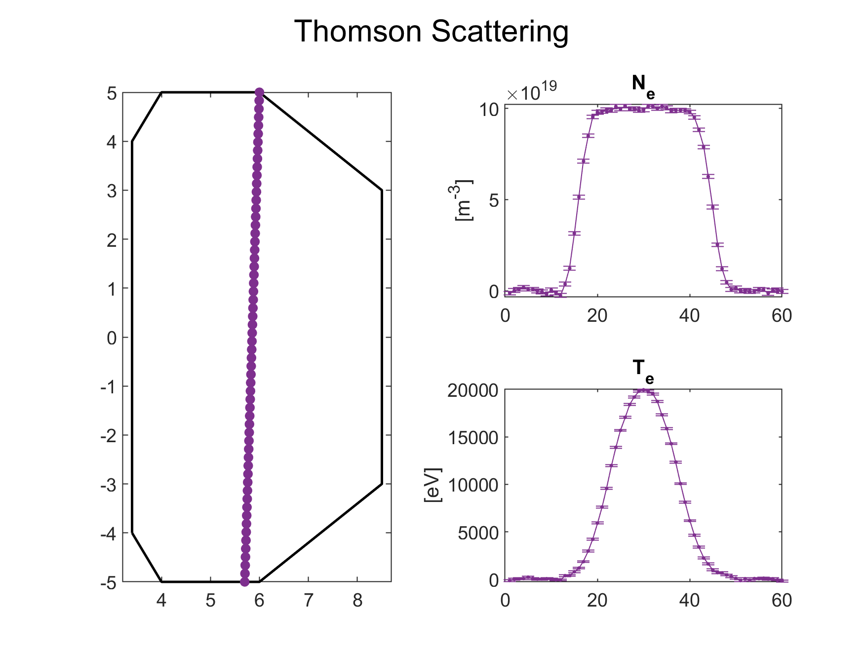
EXAMPLE 2: Modelling a vertical Thomson Scattering
In this case, a vertical Thomson Scattering has been simulated by simply changing the reference of D_TS.config.type (set, for example, to 2 in line 59 in this case) and adding an elseif condition in the ThomsonScattering.m function where it is possible to set new values for R and Z. The results obtained for the selected coordinates are shown in Figure 3.
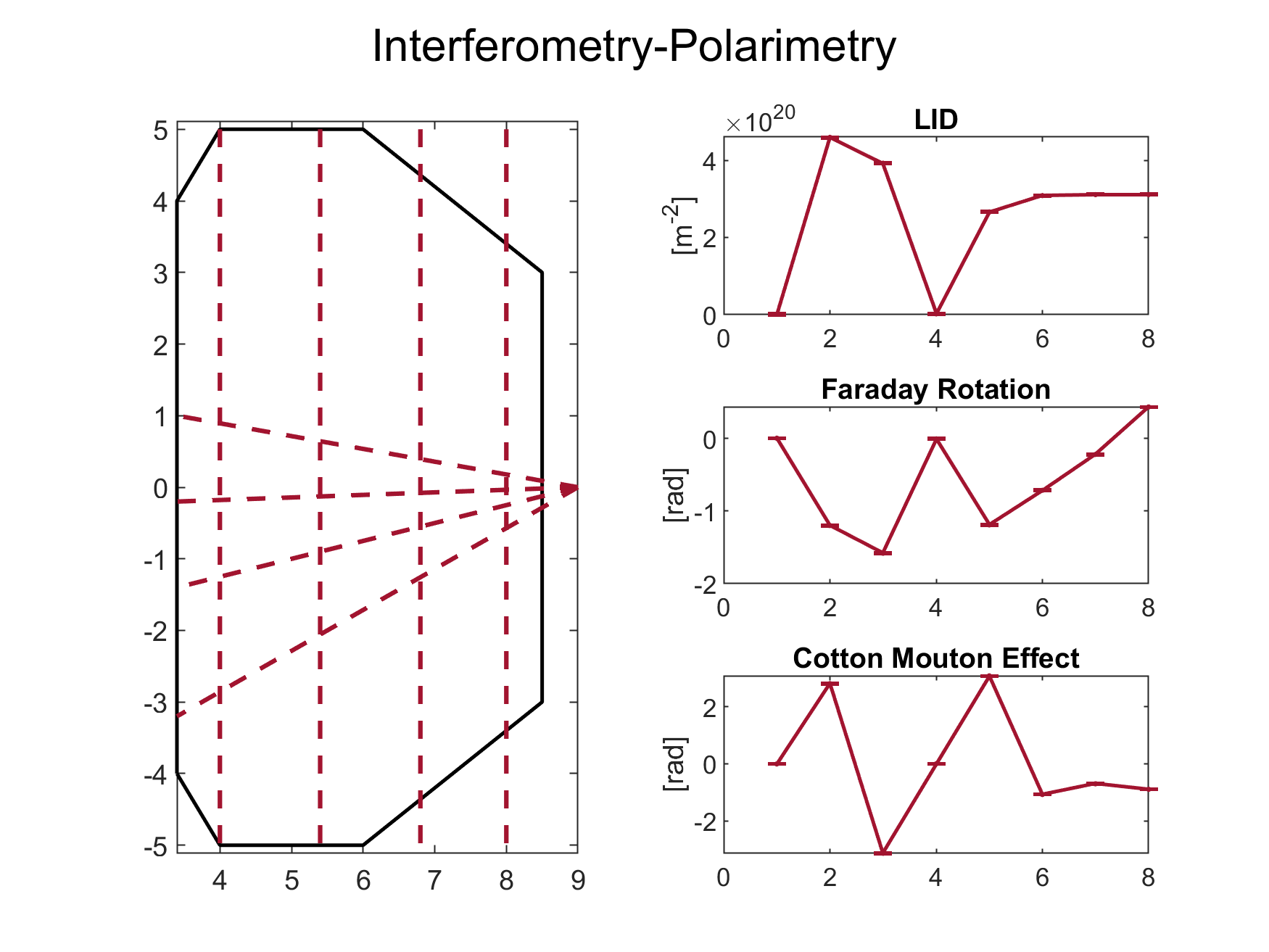
EXAMPLE 3: Changing Laser Wavelength in Interferometer-Polarimeter
This example can be useful for simulating different behaviors of polarimetric measurements at different values of λ. This can be easily done by changing the configuration type number in line 74 and adding another elseif condition in the InterferometerPolarimeter.m MATLAB function. The wavelength can be changed in line 84 of the main code, for example. The results obtained are shown in Figure 4.
Python Guide
Progresses about this guide will be released in the next future.