SimPla - Simulated Plasma
SimPla - Simulated Plasma using MATLAB_edu module
SimPla is a tool for simulating plasma behaviour using a single-fluid model in a tokamak, for example to solve a plasma equilibrium problem. In this page, a brief description to explain how to use the MATLAB_edu version, developed using a non-object oriented framework, is presented. Please note that this version is though for students approaching to plasma equilibrium, while the object oriented framework (MATLAB or Python versions) are more flexible and well-structured.
MATLAB Guide
In case you need to solve a plasma equilibrium problem, please open Main_equilibrium.m.
EXAMPLE 1: SOLVE AN ITER-LIKE CONFIGURATION
First steps require to define essential geometrical and plasma parameters of your configuration.
All geometrical parameters are collected in a structure called Geo . In Main_equilibrium.m, we define first two geometrical parameters:
-
major radius:
Geo.R0 = 6[m] -
minor radius:
Geo.a = 2[m]
%% Define Geometry (Geo)

Geo.R0 = 6;
Geo.a = 2;
All plasma equilibrium parameters are collected in the structure Equi, more specifically in its substructure Equi.Config.param.
Open Equilibrium_boundary.m, where you can input desired parameters through the function Equi_type_Jt_I_Config.m or by uploading your own file containing all data.
So, let’s now open Equi_type_Jt_I_Config.m.
First plasma equilibrium parameters are related to the desired plasma shape (for a better understanding, please refer to Appendix A), and they are:
-
upper elongation:
Equi.Config.param.k1 = 1.7 -
lower elongation:
Equi.Config.param.k2 = 2 -
upper triangularity:
Equi.Config.param.d1 = 0.5 -
lower triangularity:
Equi.Config.param.d2 = 0.5 -
upper inner angle:
Equi.Config.param.gamma_n_1 = 0[radians] -
lower inner angle:
Equi.Config.param.gamma_n_2 = pi/3[radians] -
upper outer angle:
Equi.Config.param.gamma_p_1 = 0[radians] -
lower outer angle:
Equi.Config.param.gamma_p_2 = pi/6[radians]
Other parameters are related to the plasma current profile and magnetic field:
-
total plasma current
Equi.Config.param.Ip = -10e6[A] -
plasma profile coefficient $β_0$:
Equi.Config.param.beta0 = 0.5 -
plasma profile coefficient $α_1$:
Equi.Config.param.alpha1 = 2 -
plasma profile coefficient $α_2$:
Equi.Config.param.alpha2 = 2 -
toroidal magnetic field on axis:
Equi.Config.param.Bt0 = 5;
And lastly, parameters related to the numerical solver:
-
Maximum number of iterations:
Equi.Config.param.Max_iter = 30 -
Stop condition on convergence error:
Equi.Config.param.Error_conv = 1e-5
function Equi = Equi_type_Jt_I_Config()

Equi.Config.param.k1 = 1.7;
Equi.Config.param.k2 = 2;
Equi.Config.param.d1 = 0.5;
Equi.Config.param.d2 = 0.5;
Equi.Config.param.gamma_n_1 = pi/9;
Equi.Config.param.gamma_n_2 = pi/3;
Equi.Config.param.gamma_p_1 = pi/8;
Equi.Config.param.gamma_p_2 = pi/6;

Equi.Config.param.Ip = -10e6;
Equi.Config.param.Bt0 = 5;

Equi.Config.param.Max_iter = 30;
Equi.Config.param.Error_conv = 1e-5;
Equi.Config.param.beta0 = 0.5;
Equi.Config.param.alpha1 = 2;
Equi.Config.param.alpha2 = 2;

end
Now, let’s return to Main_equilibrium.m and let’s run the code.
All equilibrium quantities are computed and stored in Equi structure.
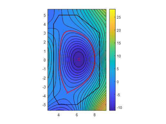
Now, we can see a plot of the poloidal flux $ψ$ [Wb/radians] (Equi.psi).
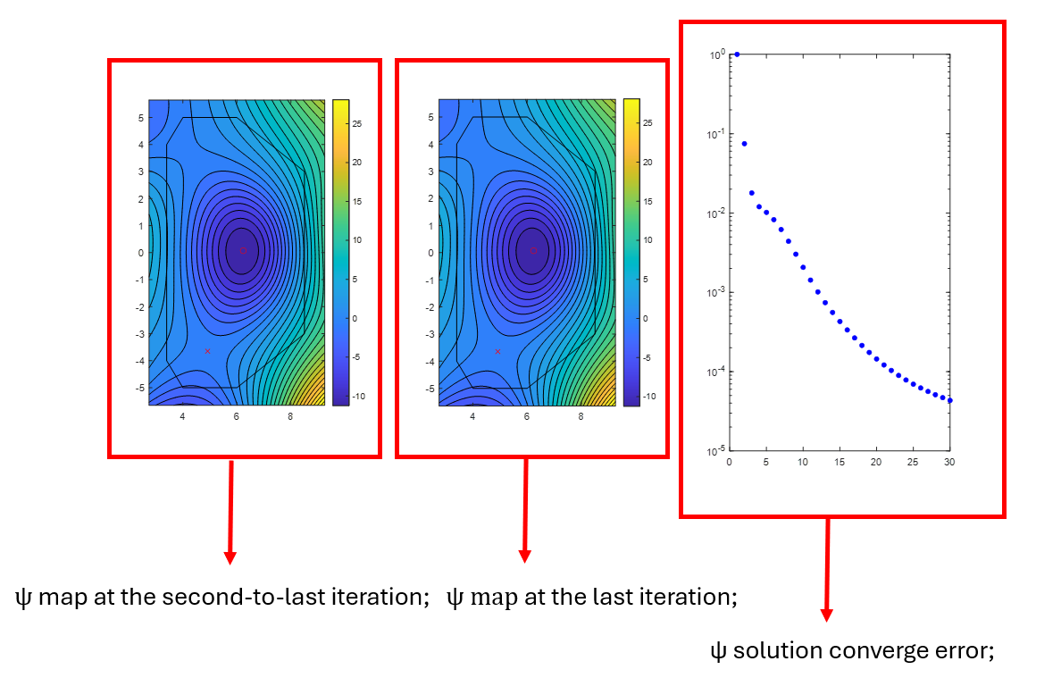
We can also see the Last Closed Flux Surface (Equi.LCFS.R, Equi.LCFS.Z) and highlight the coordinates of the magnetic axis (Equi.Opoint_R, Equi.Opoint_Z) and the X point (Equi.Xpoint_R, Equi.Xpoint_Z).
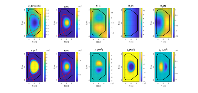
Once you normalise the poloidal flux $ψ_n$ (see Equilibrium_normalise.m), you can derive all MHD fields (Equi.Bt, Equi. Br, Equi.Bz, Equi.Jt, Equi. Jr, Equi.Jz) and kinetic fields (Equi.p, Equi.n, Equi.T).
Use Equilibrium_MHD_Fields.m function if you are interested in retrieving MHD fields and Equilibrium_KineticProfiles.m function if you are interested in kinetic fields.
Attention: before computing kinetic fields, you need to input some parameters on your plasma density profile:
-
peak plasma density $n_0$:
Equi.Config.param_kinetic.n0 = 1e20[$m^-3$] -
plasma density on the separatrix $n_{sep}$:
Equi.Config.param_kinetic.nsep = 1e17[] -
density profile double-power exponent $a_1$:
Equi.Config.param_kinetic.a1 = 6 -
density profile double-power exponent $a_2$:
Equi.Config.param_kinetic.a2 = 3
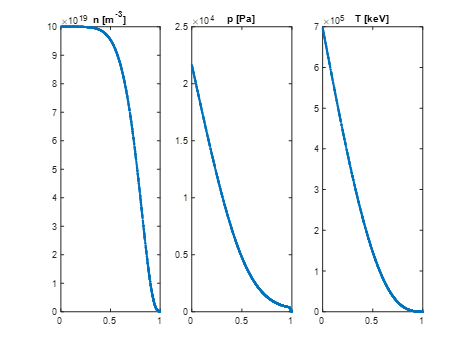
Here are some examples of the kinetic profiles n, p and T vs $\boldsymbol{\psi}_n$.
We can now also have a look at all fields that we have retrieved from the equilibrium solution.
APPENDIX A
Our reference to the parametrisation of the plasma shape is:
J. Johner, 2011, HELIOS: a zero-dimensional tool for next step and reactor studies, Fusion Sci. Technol. 59 (February) 308–349.
Here is a basic illustration of all parameters needed for the parametrisation of the desired plasma shape. Differently from our reference, angles were denoted with $\gamma$ instead of $\psi$ to avoid misinterpretation with the poloidal flux.
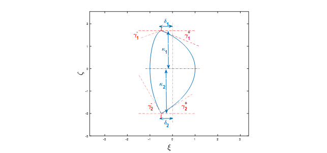
Cross-section parametrisation:
Normalised Cylindrical Coordinates:
- $ \xi = \frac{R-R_0}{a} $
- $ \zeta = \frac{Z}{a} $
Parameters:
- $ \delta_1 = $ upper triangularity
- $ \delta_2 = $ lower triangularity
- $ \kappa_1 = $ upper elongation
- $ \kappa_2 = $ lower elongation
- $ \gamma^-_1 = $ inner upper angle
- $ \gamma^-_2 = $ inner lower angle
- $ \gamma^+_1 = $ outer upper angle
- $ \gamma^+_2 = $ outer lower angle
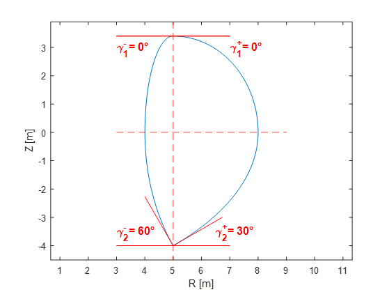
Shape example 1: Single X point ($ \gamma^-_1 = \gamma^+_1 = 0° $)
The reference for plasma toroidal current density profile is:
Coleman M. and McIntosh S., 2020, The design and optimisation of tokamak poloidal field systems in the BLUEPRINT framework, Fusion Eng. Des. 154 111544
Where $J_t$ is defined as:
\[J_t = \begin{cases} \lambda \left( \beta_0 \cdot \frac{R}{R_0} + (1 - \beta_0) \cdot \frac{R_0}{R} \right) \cdot \left(1 - \psi_n^{\alpha_1}\right)^{\alpha_2} & \text{for } 0 < \psi_n < 1 \\ 0 & \text{elsewhere} \end{cases}\]$ψ_n$ is the normalised poloidal flux $\psi_n = \frac{\psi-\psi_0}{\psi_{sep}-\psi_0}$
$λ$ and $β_0$ are parameters that affect the plasma current integral value. The shape of the profile chosen is a double power function of the normalised poloidal flux and $α_1$ and $α_2$ are the exponents of such double power function.
Python Guide
Progresses about this guide will be released in the next future.